Official Sensor Examples¶

This page shows the bundled cross-sensor example runtime built from official relative spectral response sources for Terra MODIS, Sentinel-2A MSI, Landsat 8 OLI, and Landsat 9 OLI.

It uses four held-out class targets drawn from the previously composed full SIAC library: one vegetation spectrum, one soil spectrum, one water spectrum, and one urban spectrum. Those targets are simulated to each source sensor. For each query, the examples exclude only the matching prepared row_id, leaving the rest of the external full library available.

4 sensorsMODIS, Sentinel-2A, Landsat 8, Landsat 9

4 held-out targetsvegetation, soil, water, urban

77,125 library rowsexternal full SIAC retrieval database

Example kpublic default `k = 10`

Example estimator`simplex_mixture`

Scored subsetblue, green, red, nir, swir1, swir2

Library root`build/siac_spectral_library_real_full_raw_no_ghisacasia_no_understory_no_santa37`

Regenerated2026-04-07 UTC

Related pages:

Official Sources¶

Sensor	Official source	Repository subset
Terra MODIS	NASA MCST Terra_RSR_in-band.xlsx	`examples/official_mapping/srfs/terra_modis.json`
Sentinel-2A MSI	ESA Copernicus COPE-GSEG-EOPG-TN-15-0007 - Sentinel-2 Spectral Response Functions 2024 - 4.0.xlsx	`examples/official_mapping/srfs/sentinel-2a_msi.json`
Landsat 8 OLI	USGS Spectral Characteristics Viewer band JSON	`examples/official_mapping/srfs/landsat-8_oli.json`
Landsat 9 OLI	USGS Spectral Characteristics Viewer band JSON	`examples/official_mapping/srfs/landsat-9_oli2.json`

The reduced JSON files and derived figures were regenerated from the official upstream assets on 2026-04-07 UTC. Provenance, download timestamps, and SHA-256 hashes are stored in examples/official_mapping/official_source_manifest.json.

Recorded upstream artifacts for this commit:

Terra MODIS: Terra_RSR_in-band.xlsx SHA-256 f14498183f9258ed691999313a13fc425edb2eb2d89ca676f79abbb6f48ad637
Sentinel-2A MSI: Sentinel-2_Spectral_Response_Functions_2024_4.0.xlsx SHA-256 1a9edc27d692a570911a460d589f188da0fc3e27f0b0bd1ad322059c380519b0
Landsat 8 OLI: 7 official band JSON files recorded in examples/official_mapping/official_source_manifest.json
Landsat 9 OLI: 7 official band JSON files recorded in examples/official_mapping/official_source_manifest.json

What The Example Demonstrates¶

held-out reconstruction on exact full-library spectra rather than synthetic mixtures
target-sensor mapping between MODIS, Sentinel-2A, Landsat 8, and Landsat 9
batch mapping from one CSV input
full-spectrum reconstruction over 400-2500 nm
provenance tracking for official SRF inputs

Held-Out Target Design¶

Sample id	Class	Source	Prepared row id
`blue_spruce_needles`	`vegetation`	USGS Spectral Library v7	`usgs_v7:usgs_v7_002183:Blue_Spruce DW92-5 needles BECKa AREF`
`pale_brown_silty_loam`	`soil`	ECOSTRESS Spectral Library v1.0	`ecostress_v1:ecostress_v1_002334:Pale brown silty loam`
`tap_water`	`water`	ECOSTRESS Spectral Library v1.0	`ecostress_v1:ecostress_v1_003451:Tap water`
`asphalt_road`	`urban`	USGS Spectral Library v7	`usgs_v7:usgs_v7_000004:Asphalt GDS376 Blck_Road old ASDFRa AREF`

The retrieval library itself is not vendored under examples/official_mapping because it contains 77,125 rows. Instead, the committed bundle records the expected external SIAC root and the exact held-out rows in examples/official_mapping/official_source_manifest.json.

Current full-library landcover counts:

soil: 60,905 rows
unlabeled: 5,932 rows
urban: 1,474 rows
vegetation: 8,723 rows
water: 91 rows

Each example command excludes only its own query spectrum:

single-sample runs use --exclude-row-id <row_id>
the batch input file carries an exclude_row_id column, one exact row id per query

That keeps the other held-out targets available as neighbors while still preventing self-matches.

All generated outputs on this page use k = 10 with --neighbor-estimator simplex_mixture. The overlay figure below plots the top 5 neighbors from each segment’s k = 10 retrieval for readability.

Band Correspondence¶

Semantic band	Terra MODIS	Sentinel-2A MSI	Landsat 8 OLI	Landsat 9 OLI
`ultra_blue`	not present	`B1`	`Band 1`	`Band 1`
`blue`	`Band 3`	`B2`	`Band 2`	`Band 2`
`green`	`Band 4`	`B3`	`Band 3`	`Band 3`
`red`	`Band 1`	`B4`	`Band 4`	`Band 4`
`nir`	`Band 2`	`B08`	`Band 5`	`Band 5`
`swir1`	`Band 6`	`B11`	`Band 6`	`Band 6`
`swir2`	`Band 7`	`B12`	`Band 7`	`Band 7`

Sentinel-2 is represented here by the S2A sheet from the official ESA SRF workbook. If you need S2B or S2C, the same conversion script can be pointed at the corresponding official sheet.

Rebuild The Example Bundle¶

Regenerate the sensor JSON, example queries, results, and plot assets:

python3 -m pip install ".[internal-build]"
python3 scripts/build_official_mapping_examples.py --siac-root build/siac_spectral_library_real_full_raw_no_ghisacasia_no_understory_no_santa37

That script downloads the official source assets, writes the reduced sensor schemas into examples/official_mapping/srfs, rebuilds the example queries and outputs against the external full SIAC library, refreshes the figures in docs/assets, and rewrites this page from the generated outputs. It requires network access for the upstream SRF files and expects the full SIAC library to already exist at build/siac_spectral_library_real_full_raw_no_ghisacasia_no_understory_no_santa37 or at the path passed by --siac-root.

Prepare The Runtime¶

Use the previously composed full SIAC library and the official-source SRF JSONs:

spectral-library build-mapping-library \
  --siac-root build/siac_spectral_library_real_full_raw_no_ghisacasia_no_understory_no_santa37 \
  --srf-root examples/official_mapping/srfs \
  --source-sensor terra_modis \
  --source-sensor sentinel-2a_msi \
  --source-sensor landsat-8_oli \
  --source-sensor landsat-9_oli2 \
  --output-root build/official_mapping_runtime

Validate the prepared runtime:

spectral-library validate-prepared-library \
  --prepared-root build/official_mapping_runtime

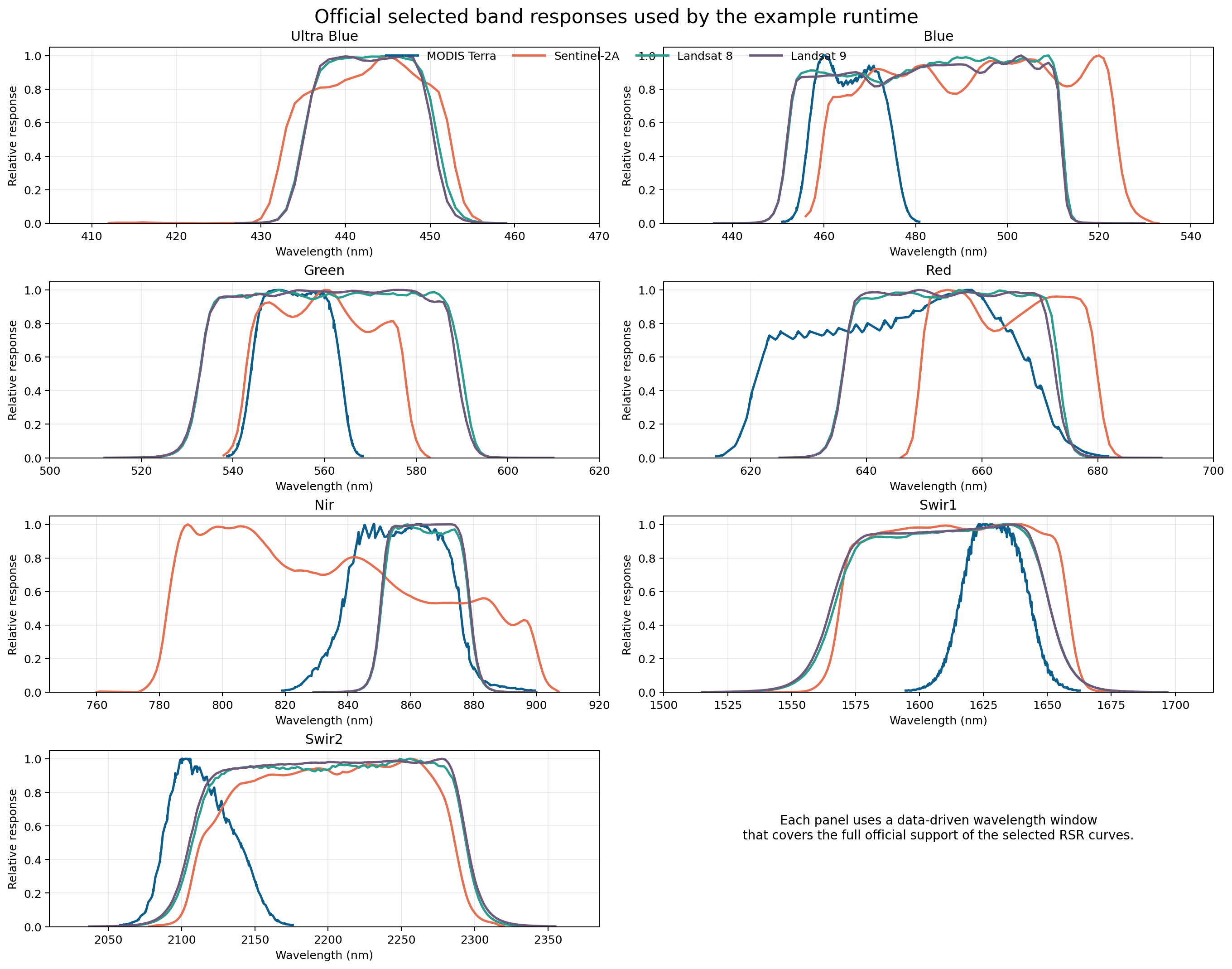
Visual Comparison¶

Selected official band responses used by the example runtime:

Selected official band responses

Mean absolute target-band error across the four held-out class targets, evaluated only on the common comparable subset blue, green, red, nir, swir1, swir2:

Pairwise mapping error

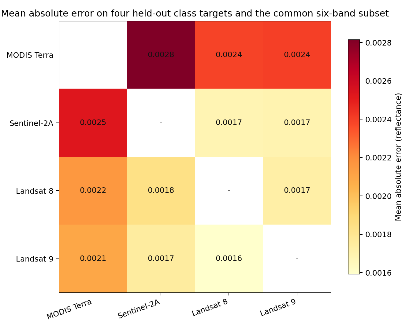
Observed range in the bundled example:

lowest comparable mean absolute band error: 0.0016 for Landsat 9 -> Landsat 8
highest comparable mean absolute band error: 0.0028 for MODIS Terra -> Sentinel-2A
pairwise metrics on this page were generated with neighbor_estimator = simplex_mixture

The full pairwise summary, including evaluated_band_ids and evaluated_band_count, is in examples/official_mapping/results/metrics/pairwise_band_metrics.csv.

Held-Out Estimator Comparison¶

The full-library held-out benchmark compares mean, distance_weighted_mean, and simplex_mixture on the four exact public targets across all 12 ordered source-target pairs.

Held-out estimator comparison

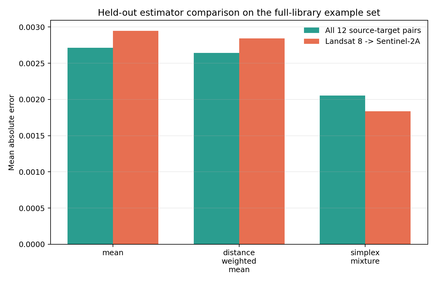
best aggregate held-out mean absolute error: 0.0021 with simplex_mixture
best Landsat 8 -> Sentinel-2A held-out mean absolute error: 0.0018 with simplex_mixture

Reference benchmark files:

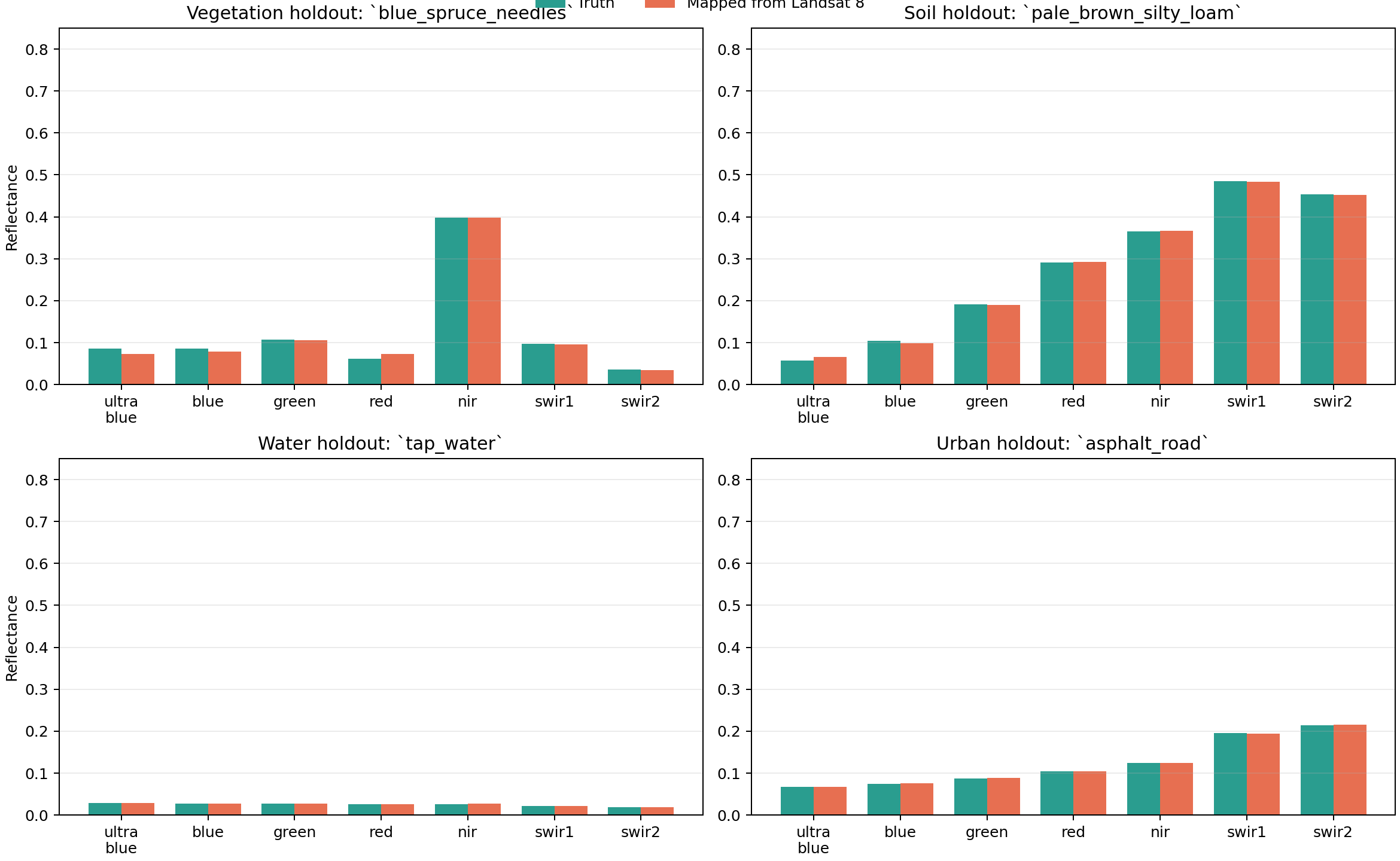
Held-out Landsat 8 to Sentinel-2A batch comparison across vegetation, soil, water, and urban targets:

Held-out batch comparison

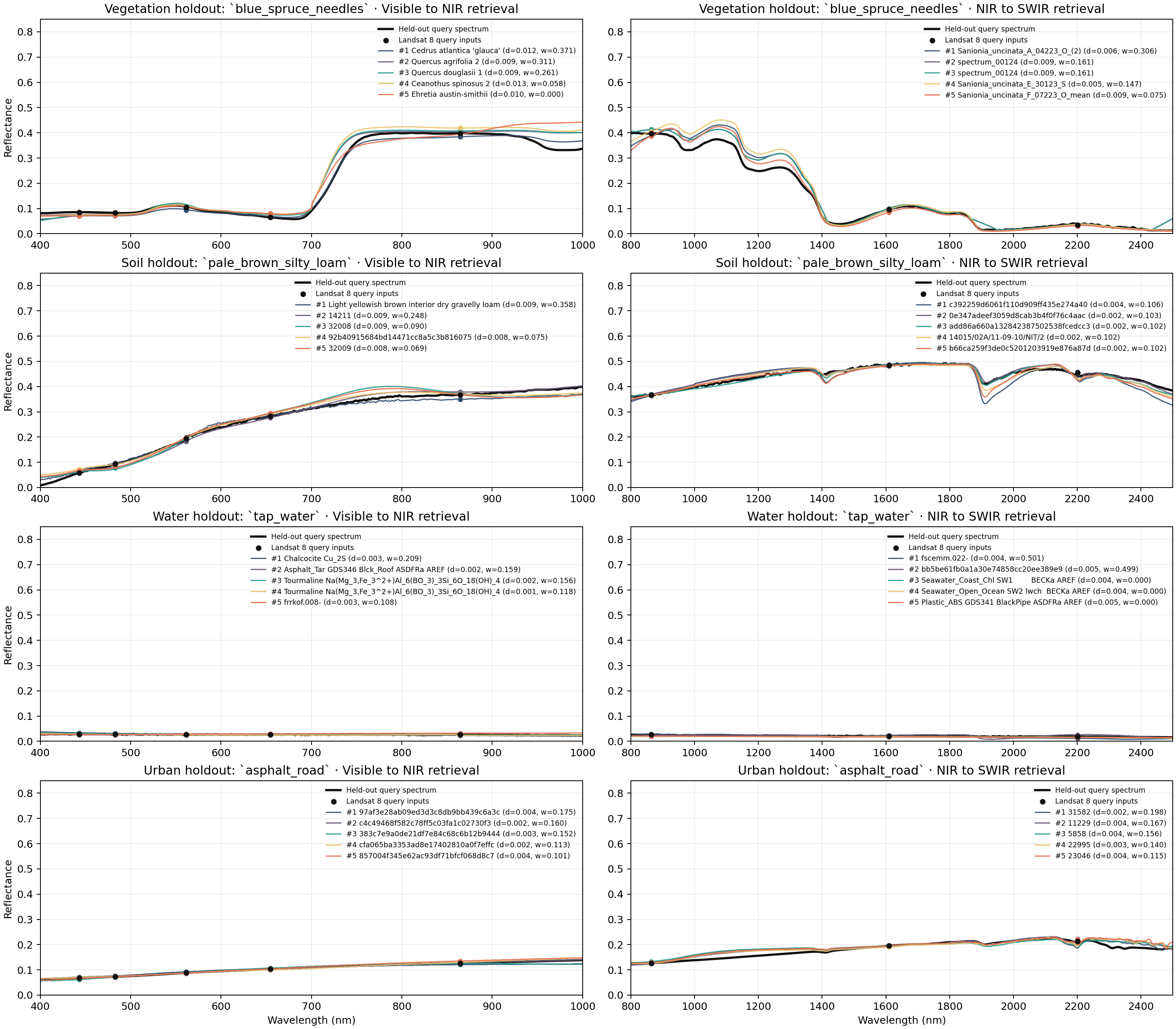
Neighbor Overlay Diagnostic¶

The figure below shows the two retrievals independently for each held-out Landsat 8 query:

left panel: the visible-to-NIR retrieval over 400-1000 nm
right panel: the NIR-to-SWIR retrieval over 800-2500 nm

Even when the input query includes all Landsat 8 reflective bands, the runtime does not do one joint KNN search across the entire source vector. It always builds two query vectors, retrieves neighbors independently for each segment, and only then combines the reconstructed segments into the final full-spectrum product.

Each panel overlays:

the held-out hyperspectral query spectrum
the segment-specific Landsat 8 query inputs used in that retrieval
the top 5 weighted neighbors from the segment’s k = 10 shortlist on the full library, labeled with source-space distance and estimator weight

This makes one important behavior explicit: KNN is query-centric within each segment. It ranks candidates by distance to that segment’s query features, but it does not require the neighbors to be mutually similar or to share the same landcover label. The simplex_mixture estimator then reweights that shortlist to fit the query within the convex hull of the retrieved source-band vectors.

Holdout neighbor overlays

The table below is generated directly from the committed batch diagnostics JSON. It shows the top weighted neighbors used by the estimator for each sample and segment, together with their source-space distance, simplex weight, and the actual source-band values seen by the fit.

Sample	Segment	Rank	Neighbor	Distance	Weight	Source-fit RMSE	Query values	Neighbor source-band values
`asphalt_road`	`vnir`	`7`	`97af3e28ab09ed3d3c8db9bb439c6a3c`	`0.0037`	`0.1748`	`0.0005`	`ultra_blue=0.0677, blue=0.0731, green=0.0883, red=0.1032, nir=0.1266`	`ultra_blue=0.0710, blue=0.0762, green=0.0920, red=0.1036, nir=0.1207`
`asphalt_road`	`vnir`	`2`	`c4c49468f582c78ff5c03fa1c02730f3`	`0.0024`	`0.1603`	`0.0005`	`ultra_blue=0.0677, blue=0.0731, green=0.0883, red=0.1032, nir=0.1266`	`ultra_blue=0.0712, blue=0.0759, green=0.0865, red=0.1008, nir=0.1267`
`asphalt_road`	`vnir`	`5`	`383c7e9a0de21df7e84c68c6b12b9444`	`0.0034`	`0.1518`	`0.0005`	`ultra_blue=0.0677, blue=0.0731, green=0.0883, red=0.1032, nir=0.1266`	`ultra_blue=0.0617, blue=0.0713, green=0.0889, red=0.1071, nir=0.1250`
`asphalt_road`	`swir`	`1`	`31582`	`0.0016`	`0.1976`	`0.0021`	`nir=0.1266, swir1=0.1951, swir2=0.2139`	`nir=0.1292, swir1=0.1945, swir2=0.2132`
`asphalt_road`	`swir`	`9`	`11229`	`0.0045`	`0.1672`	`0.0021`	`nir=0.1266, swir1=0.1951, swir2=0.2139`	`nir=0.1245, swir1=0.1933, swir2=0.2211`
`asphalt_road`	`swir`	`5`	`5858`	`0.0039`	`0.1558`	`0.0021`	`nir=0.1266, swir1=0.1951, swir2=0.2139`	`nir=0.1328, swir1=0.1955, swir2=0.2113`
`blue_spruce_needles`	`vnir`	`6`	`Cedrus atlantica 'glauca'`	`0.0116`	`0.3705`	`0.0078`	`ultra_blue=0.0857, blue=0.0836, green=0.1036, red=0.0656, nir=0.3978`	`ultra_blue=0.0703, blue=0.0722, green=0.0932, red=0.0690, nir=0.3843`
`blue_spruce_needles`	`vnir`	`1`	`Quercus agrifolia 2`	`0.0087`	`0.3108`	`0.0078`	`ultra_blue=0.0857, blue=0.0836, green=0.1036, red=0.0656, nir=0.3978`	`ultra_blue=0.0761, blue=0.0781, green=0.1075, red=0.0796, nir=0.4046`
`blue_spruce_needles`	`vnir`	`2`	`Quercus douglasii 1`	`0.0092`	`0.2608`	`0.0078`	`ultra_blue=0.0857, blue=0.0836, green=0.1036, red=0.0656, nir=0.3978`	`ultra_blue=0.0736, blue=0.0773, green=0.1100, red=0.0758, nir=0.4073`
`blue_spruce_needles`	`swir`	`2`	`Sanionia_uncinata_A_04223_O_(2)`	`0.0062`	`0.3057`	`0.0016`	`nir=0.3978, swir1=0.0956, swir2=0.0350`	`nir=0.3872, swir1=0.0944, swir2=0.0334`
`blue_spruce_needles`	`swir`	`5`	`spectrum_00124`	`0.0088`	`0.1608`	`0.0016`	`nir=0.3978, swir1=0.0956, swir2=0.0350`	`nir=0.4125, swir1=0.0990, swir2=0.0332`
`blue_spruce_needles`	`swir`	`6`	`spectrum_00124`	`0.0088`	`0.1608`	`0.0016`	`nir=0.3978, swir1=0.0956, swir2=0.0350`	`nir=0.4125, swir1=0.0990, swir2=0.0332`
`pale_brown_silty_loam`	`vnir`	`8`	`Light yellowish brown interior dry gravelly loam`	`0.0091`	`0.3583`	`0.0044`	`ultra_blue=0.0581, blue=0.0937, green=0.1935, red=0.2837, nir=0.3678`	`ultra_blue=0.0644, blue=0.0977, green=0.1983, red=0.2854, nir=0.3496`
`pale_brown_silty_loam`	`vnir`	`9`	`14211`	`0.0094`	`0.2478`	`0.0044`	`ultra_blue=0.0581, blue=0.0937, green=0.1935, red=0.2837, nir=0.3678`	`ultra_blue=0.0657, blue=0.0842, green=0.1822, red=0.2767, nir=0.3786`
`pale_brown_silty_loam`	`vnir`	`7`	`32008`	`0.0090`	`0.0904`	`0.0044`	`ultra_blue=0.0581, blue=0.0937, green=0.1935, red=0.2837, nir=0.3678`	`ultra_blue=0.0624, blue=0.0782, green=0.1921, red=0.2949, nir=0.3718`
`pale_brown_silty_loam`	`swir`	`10`	`c392259d6061f110d909ff435e274a40`	`0.0038`	`0.1057`	`0.0008`	`nir=0.3678, swir1=0.4842, swir2=0.4543`	`nir=0.3641, swir1=0.4877, swir2=0.4502`
`pale_brown_silty_loam`	`swir`	`6`	`0e347adeef3059d8cab3b4f0f76c4aac`	`0.0025`	`0.1032`	`0.0008`	`nir=0.3678, swir1=0.4842, swir2=0.4543`	`nir=0.3691, swir1=0.4822, swir2=0.4579`
`pale_brown_silty_loam`	`swir`	`2`	`add86a660a132842387502538fcedcc3`	`0.0015`	`0.1023`	`0.0008`	`nir=0.3678, swir1=0.4842, swir2=0.4543`	`nir=0.3693, swir1=0.4833, swir2=0.4562`
`tap_water`	`vnir`	`7`	`Chalcocite Cu_2S`	`0.0031`	`0.2094`	`0.0001`	`ultra_blue=0.0286, blue=0.0279, green=0.0270, red=0.0265, nir=0.0262`	`ultra_blue=0.0338, blue=0.0313, green=0.0286, red=0.0280, nir=0.0239`
`tap_water`	`vnir`	`5`	`Asphalt_Tar GDS346 Blck_Roof ASDFRa AREF`	`0.0022`	`0.1587`	`0.0001`	`ultra_blue=0.0286, blue=0.0279, green=0.0270, red=0.0265, nir=0.0262`	`ultra_blue=0.0257, blue=0.0255, green=0.0252, red=0.0248, nir=0.0241`
`tap_water`	`vnir`	`3`	`Tourmaline Na(Mg_3,Fe_3^2+)Al_6(BO_3)_3Si_6O_18(OH)_4`	`0.0017`	`0.1556`	`0.0001`	`ultra_blue=0.0286, blue=0.0279, green=0.0270, red=0.0265, nir=0.0262`	`ultra_blue=0.0314, blue=0.0300, green=0.0283, red=0.0268, nir=0.0259`
`tap_water`	`swir`	`3`	`fscemm.022-`	`0.0045`	`0.5008`	`0.0004`	`nir=0.0262, swir1=0.0210, swir2=0.0189`	`nir=0.0284, swir1=0.0191, swir2=0.0117`
`tap_water`	`swir`	`5`	`bb5be61fb0a1a30e74858cc20ee389e9`	`0.0045`	`0.4992`	`0.0004`	`nir=0.0262, swir1=0.0210, swir2=0.0189`	`nir=0.0230, swir1=0.0237, swir2=0.0255`
`tap_water`	`swir`	`1`	`Seawater_Coast_Chl SW1 BECKa AREF`	`0.0042`	`0.0000`	`0.0004`	`nir=0.0262, swir1=0.0210, swir2=0.0189`	`nir=0.0198, swir1=0.0186, swir2=0.0163`

Single-Sample Mapping Runs¶

MODIS Terra to Sentinel-2A on the vegetation holdout:

spectral-library map-reflectance \
  --prepared-root build/official_mapping_runtime \
  --source-sensor terra_modis \
  --target-sensor sentinel-2a_msi \
  --input examples/official_mapping/queries/single/blue_spruce_needles_terra_modis.csv \
  --output-mode target_sensor \
  --neighbor-estimator simplex_mixture \
  --exclude-row-id 'usgs_v7:usgs_v7_002183:Blue_Spruce DW92-5 needles    BECKa AREF' \
  --output build/official_mapping_runtime/blue_spruce_needles_modis_to_sentinel2a.csv

Reference output: examples/official_mapping/results/selected/blue_spruce_needles_modis_to_sentinel2a.csv

Band	Truth	Mapped
`ultra_blue`	`0.0856`	`0.0721`
`blue`	`0.0858`	`0.0778`
`green`	`0.1065`	`0.1066`
`red`	`0.0621`	`0.0722`
`nir`	`0.3979`	`0.3978`
`swir1`	`0.0971`	`0.0954`
`swir2`	`0.0356`	`0.0331`

The ultra_blue band is shown in the example table because it is a real target output for Sentinel-2A, but it is intentionally excluded from the pairwise heatmap so every source-target cell is scored on the same comparable six-band subset.

Sentinel-2A to Landsat 9 on the soil holdout:

spectral-library map-reflectance \
  --prepared-root build/official_mapping_runtime \
  --source-sensor sentinel-2a_msi \
  --target-sensor landsat-9_oli2 \
  --input examples/official_mapping/queries/single/pale_brown_silty_loam_sentinel-2a_msi.csv \
  --output-mode target_sensor \
  --neighbor-estimator simplex_mixture \
  --exclude-row-id 'ecostress_v1:ecostress_v1_002334:Pale brown silty loam' \
  --output build/official_mapping_runtime/pale_brown_silty_loam_sentinel2a_to_landsat9.csv

Reference output: examples/official_mapping/results/selected/pale_brown_silty_loam_sentinel2a_to_landsat9.csv

Landsat 8 to MODIS on the urban holdout:

spectral-library map-reflectance \
  --prepared-root build/official_mapping_runtime \
  --source-sensor landsat-8_oli \
  --target-sensor terra_modis \
  --input examples/official_mapping/queries/single/asphalt_road_landsat-8_oli.csv \
  --output-mode target_sensor \
  --neighbor-estimator simplex_mixture \
  --exclude-row-id 'usgs_v7:usgs_v7_000004:Asphalt GDS376 Blck_Road old ASDFRa AREF' \
  --output build/official_mapping_runtime/asphalt_road_landsat8_to_modis.csv

Reference output: examples/official_mapping/results/selected/asphalt_road_landsat8_to_modis.csv

Batch Example¶

The bundled batch CSV uses Landsat 8 as the source sensor for the four held-out targets:

spectral-library map-reflectance-batch \
  --prepared-root build/official_mapping_runtime \
  --source-sensor landsat-8_oli \
  --target-sensor sentinel-2a_msi \
  --input examples/official_mapping/queries/batch/landsat8_holdout_batch.csv \
  --output-mode target_sensor \
  --neighbor-estimator simplex_mixture \
  --output build/official_mapping_runtime/landsat8_to_sentinel2a_holdout_batch.csv \
  --diagnostics-output build/official_mapping_runtime/landsat8_to_sentinel2a_holdout_batch_diagnostics.json \
  --neighbor-review-output build/official_mapping_runtime/landsat8_to_sentinel2a_holdout_neighbor_review.csv

The batch input file examples/official_mapping/queries/batch/landsat8_holdout_batch.csv includes an exclude_row_id column, so each query removes only its own exact prepared row from the shared full-library runtime.

Reference output: examples/official_mapping/results/selected/landsat8_to_sentinel2a_holdout_batch.csv

Reference diagnostics: examples/official_mapping/results/selected/landsat8_to_sentinel2a_holdout_batch_diagnostics.json

Reference neighbor review: examples/official_mapping/results/selected/landsat8_to_sentinel2a_holdout_neighbor_review.csv

Full-Spectrum Reconstruction¶

Reconstruct the full 400-2500 nm spectrum from the water holdout:

spectral-library map-reflectance \
  --prepared-root build/official_mapping_runtime \
  --source-sensor sentinel-2a_msi \
  --input examples/official_mapping/queries/single/tap_water_sentinel-2a_msi.csv \
  --output-mode full_spectrum \
  --neighbor-estimator simplex_mixture \
  --exclude-row-id 'ecostress_v1:ecostress_v1_003451:Tap water' \
  --output build/official_mapping_runtime/tap_water_sentinel2a_full_spectrum.csv

Reference output: examples/official_mapping/results/selected/tap_water_sentinel2a_full_spectrum.csv